The Transformer review
The article The Illustrated Transformer by J. Alammar is a must read on deep learning in the field of natural language processing (NLP). Also, this was recommended in one of the expert interview that I conducted.
Review of Attention
- Attention is a concept that helped improve the performance of neural machine translation applications. An attention model differs from a classic sequence-to-sequence model in two main ways:
- First, the encoder passes a lot more data to the decoder. Instead of passing the last hidden state of the encoding stage, the encoder passes all the hidden states to the decoder.
- Second, an attention decoder does an extra step before producing its output. In order to focus on the parts of the input that are relevant to this decoding time step.
- The transformer is a model that uses attention to boost the speed with which these models can be trained.
A High-Level Look
- The transformer consists of an encoding component, a decoding component, and connections between them.
- The encoding component os a stack of encoders, the decoding component is a stack of decoders of the same number.
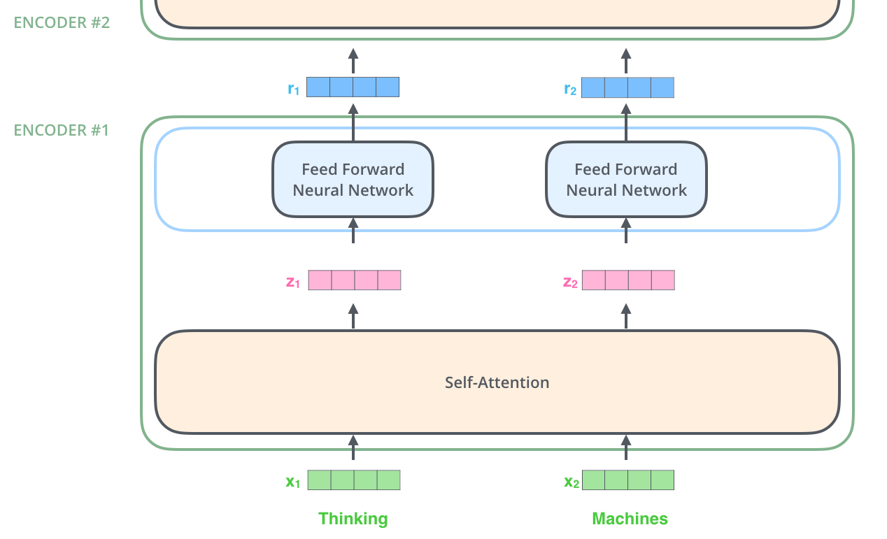
- The encoders are all identical in structure (but do not share weights). Each consists of a ‘Feed Forward Neural Network’ (ffn) and a ‘Self-Attention’ (sa) layer.
- The encoder’s input first flows through a self-attention layer - which helps the encoder to look at other words in the input sentence as it encodes a specific word.
- The encoder’s outputs of the ‘Self-Attention’ layer are feed to the ‘Feed Forward Neural Network’. The exact same ffn is independently applied to each position.
- The decoder has also the ffn and the sa layer but in between there is an ‘Encoder-Decoder Attention’ layer. This layer helps the decoder focus on relevant parts of the input sentence.
Bringing Tensors into the Picture
- The various vectors/tensors flow between these components to turn the input of a trained model into an output. This begins with turning each input word into a vector using an embedding algorithm.
- The embedding happens only in the first (bottom-most) encoder. The abstraction that is common to all encoders is that they receive a list of vectors each of the size 512. The size of the list is a hyperparameter, i.e. the length of the longest sentence in the training dataset.
- in the bottom encoder that is the word embeddings.
- in other encoders it is the output of the previous encoder.
- After embedding the words in the input sequence, each of them flows through each of the two layers of the encoder. Each word in each position flows through its own path in the encoder. There are dependencies between these paths in the sa layer. The ffn layer does not have these dependencies which is why they various paths can be executed in parallel.
Self-Attention at a High Level
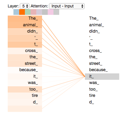
- ”The animal didn’t cross the street because it was too tired”. What does ‘it’ in the sentence refer to? The street or the animal?
- When the model is processing the word “it”, self-attention allows it to associate “it” with “animal”. As the model processes each word (each position in the input sequence), self attention allows it to look at other positions in the input sequence for clues that can help lead to a better encoding for this word.
Self-Attention in Detail
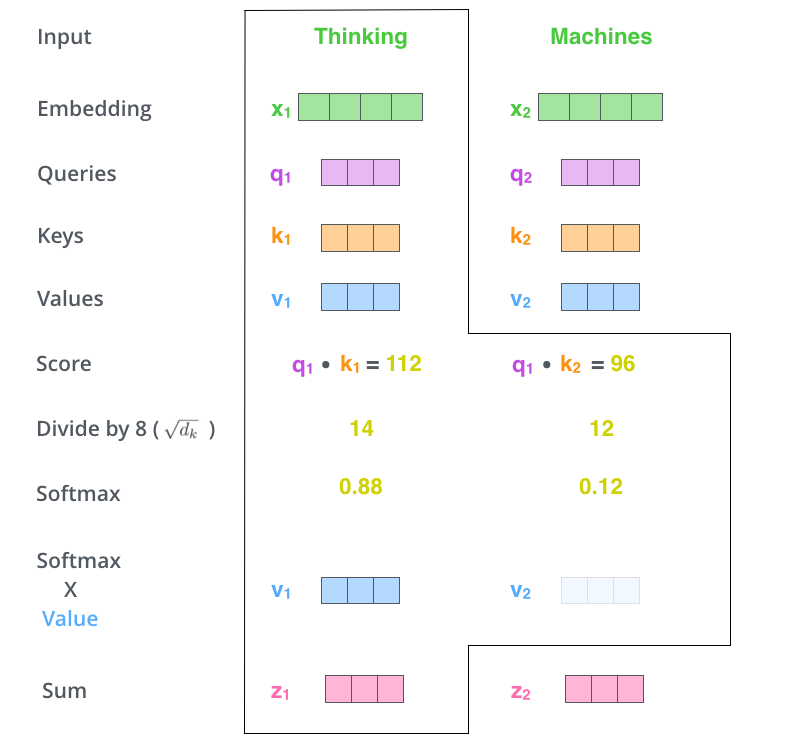
- The first step in calculating self-attention is to create three vectors from each of the encoder’s input vectors (embedding of each word). So for each word:
- we create a Query vector,
- a Key vector, and
- a Value vector.
- These vectors are created by multiplying the embedding by three matrices that we trained during the training process.
- The second step is to calculate a score. We need to score each word of the input sentence against a word. The score determines how much focus to place on other parts of the input sentence as we encode a word at a certain position.
- The score is calculated by taking the dot product of the query vector with the key vector of the respective word we’re scoring.
- So if we’re processing the self-attention for the word in position 1, the first score would be the dot product of q1 and k1. The second score would be the dot product of q1 and k2.
- The third step is to divide the scores by 8. This leads to having more stable gradients.
- The fourth step is to pass the result through a softmax operation. Softmax normalizes the scores so they’re all positive and add up to 1. This softmax score determines how much each word will be expressed at this position.
- The fifth step is to multiply each value vector by the softmax score (in preparation to sum them up). The intuition is to keep intact the values of the word(s) we want to focus on, and drown-out irrelevant.
- The sixth step is to sum the weighted value vectors. This produces the output of the self-attention layer at this position.
- The result will be sent along to the ffn network.
Matrix Calculation of Self-attention
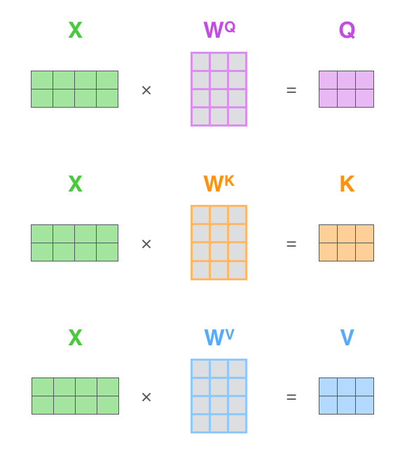
- The first step is to calculate the Query, Key, and Value matrices. We do that by packing our embeddings into a matrix X, and multiplying it by the weight matrices we’ve trained (WQ, WK, WV).
- Every row in the X matrix corresponds to a word in the input sentence. We again see the difference in size of the embedding vector (512, or 4 boxes in the figure), and the q/k/v vectors (64, or 3 boxes in the figure):
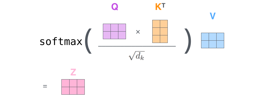
- Finally, since we’re dealing with matrices, we can condense steps two through six in one formula to calculate the outputs of the self-attention layer.
The Beast with Many Heads
- Multi-headed attention improves sa layer in two ways:
- It expands the model’s ability to focus on different positions. We would want to know which word “it” refers to.
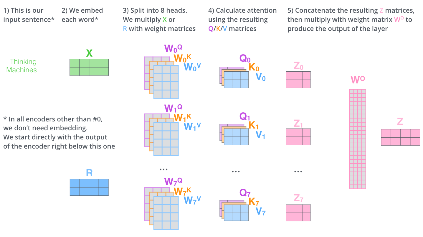
- It gives the attention layer multiple “representation subspaces”. With multi-headed attention we have not only one, but multiple sets of Query/Key/Value weight matrices . Each of these sets is randomly initialized. Then, after training, each set is used to project the input embeddings (or vectors from lower encoders/decoders) into a different representation subspace.
- If we do the same self-attention calculation we outlined above, just eight different times with different weight matrices, we end up with eight different Z matrices. Yet, the feed-forward layer is not expecting eight matrices – it’s expecting a single matrix (a vector for each word).Therefore, we concat the matrices then multiple them by an additional weights matrix WO.
Representing The Order of The Sequence Using Positional Encoding
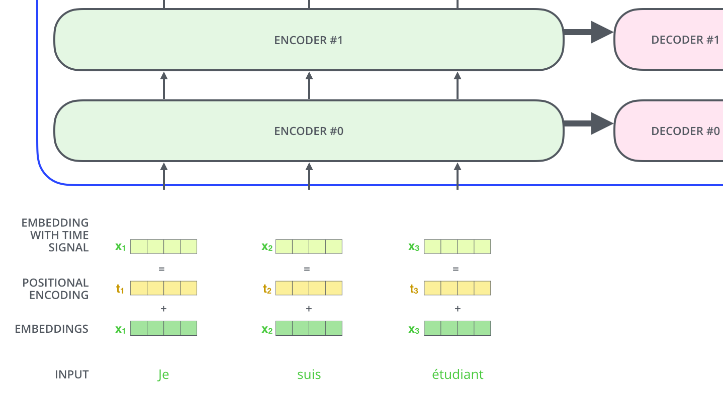
- One thing that’s missing from the model as we have described it so far is a way to account for the order of the words in the input sequence. To address this, the transformer adds a vector to each input embedding. These vectors follow a specific pattern that the model learns, which helps it determine the position of each word, or the distance between different words in the sequence. The intuition here is that adding these values to the embeddings provides meaningful distances between the embedding vectors once they’re projected into Q/K/V vectors and during dot-product attention.
The Residuals
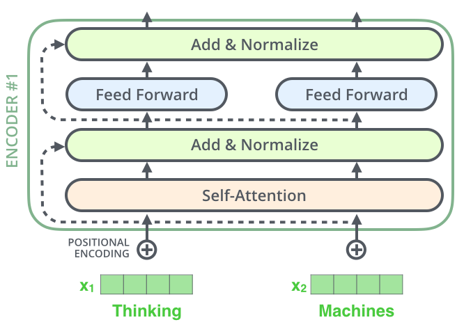
- One detail in the architecture of the encoder that we need to mention before moving on, is that each sub-layer (self-attention, ffnn) in each encoder has a residual connection around it, and is followed by a layer-normalization step.
The Decoder Side
The encoder start by processing the input sequence. The output of the top encoder is then transformed into a set of attention vectors K and V. These are to be used by each decoder in its “encoder-decoder attention” layer which helps the decoder focus on appropriate places in the input sequence.
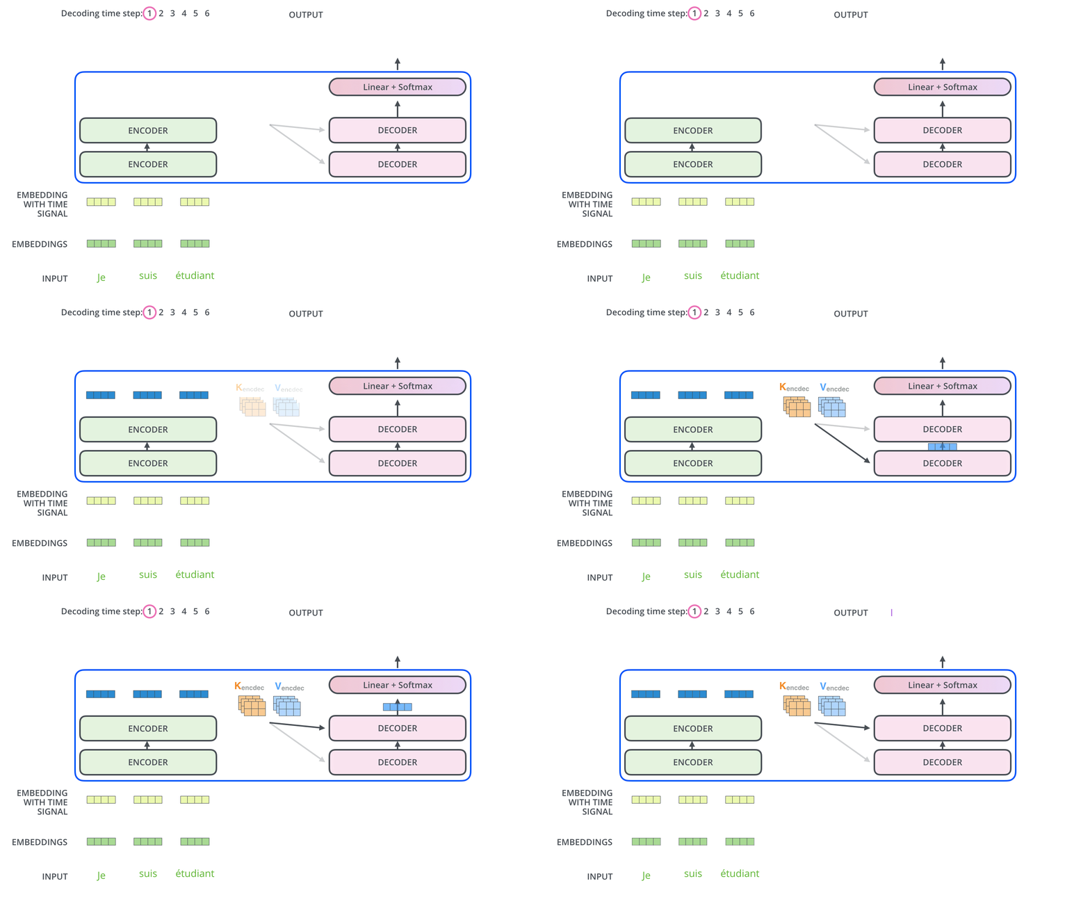
The following steps repeat the process until a special symbol is reached indicating the transformer decoder has completed its output. The output of each step is fed to the bottom decoder in the next time step, and the decoders bubble up their decoding results just like the encoders did. And just like we did with the encoder inputs, we embed and add positional encoding to those decoder inputs to indicate the position of each word.
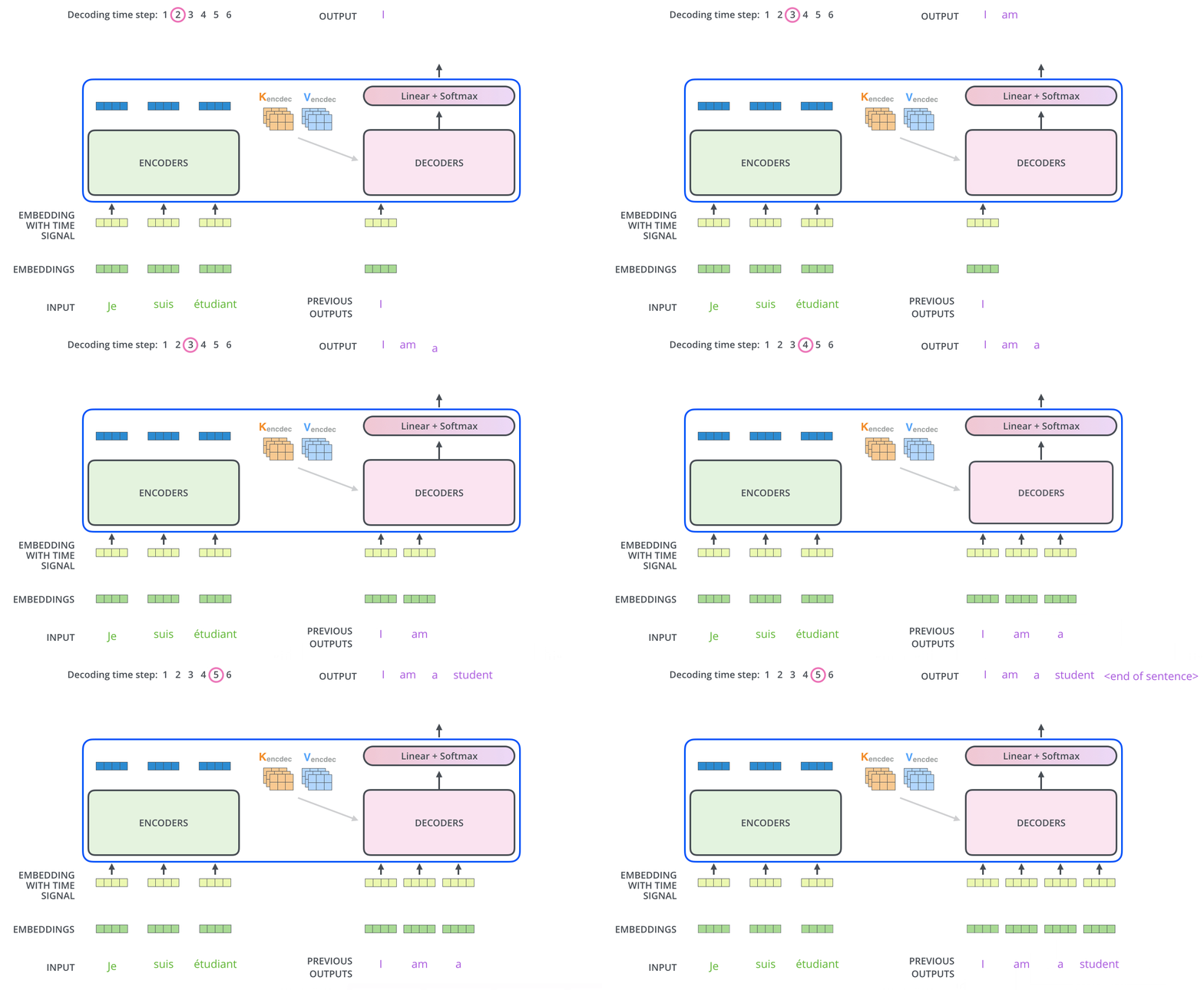
In the decoder, the self-attention layer is only allowed to attend to earlier positions in the output sequence. This is done by masking future positions (setting them to -inf) before the softmax step in the self-attention calculation.
The “Encoder-Decoder Attention” layer works just like multiheaded self-attention, except it creates its Queries matrix from the layer below it, and takes the Keys and Values matrix from the output of the encoder stack.
The Final Linear and Softmax Layer
The decoder stack outputs a vector of floats. How do we turn that into a word? That’s the job of the final Linear layer which is followed by a Softmax Layer.
The Linear layer is a simple fully connected neural network that projects the vector produced by the stack of decoders, into a much, much larger vector called a logits vector.
Let’s assume that our model knows 10,000 unique English words (our model’s “output vocabulary”) that it’s learned from its training dataset. This would make the logits vector 10,000 cells wide – each cell corresponding to the score of a unique word. That is how we interpret the output of the model followed by the Linear layer.
The softmax layer then turns those scores into probabilities (all positive, all add up to 1.0). The cell with the highest probability is chosen, and the word associated with it is produced as the output for this time step.